Gradient Descent, with Math and Jupyter

Gradient descent is an iterative method for minimizing a function. It appears in linear regression, neural-network training, and many other optimization problems. The central idea is simple: calculate which direction makes the objective increase fastest, then take a step in the opposite direction.

This article introduces the math and accompanies a runnable Jupyter notebook with NumPy implementations and Matplotlib visualizations. Download the notebook and open it in JupyterLab, classic Jupyter Notebook, or VS Code with the Python and Jupyter extensions.

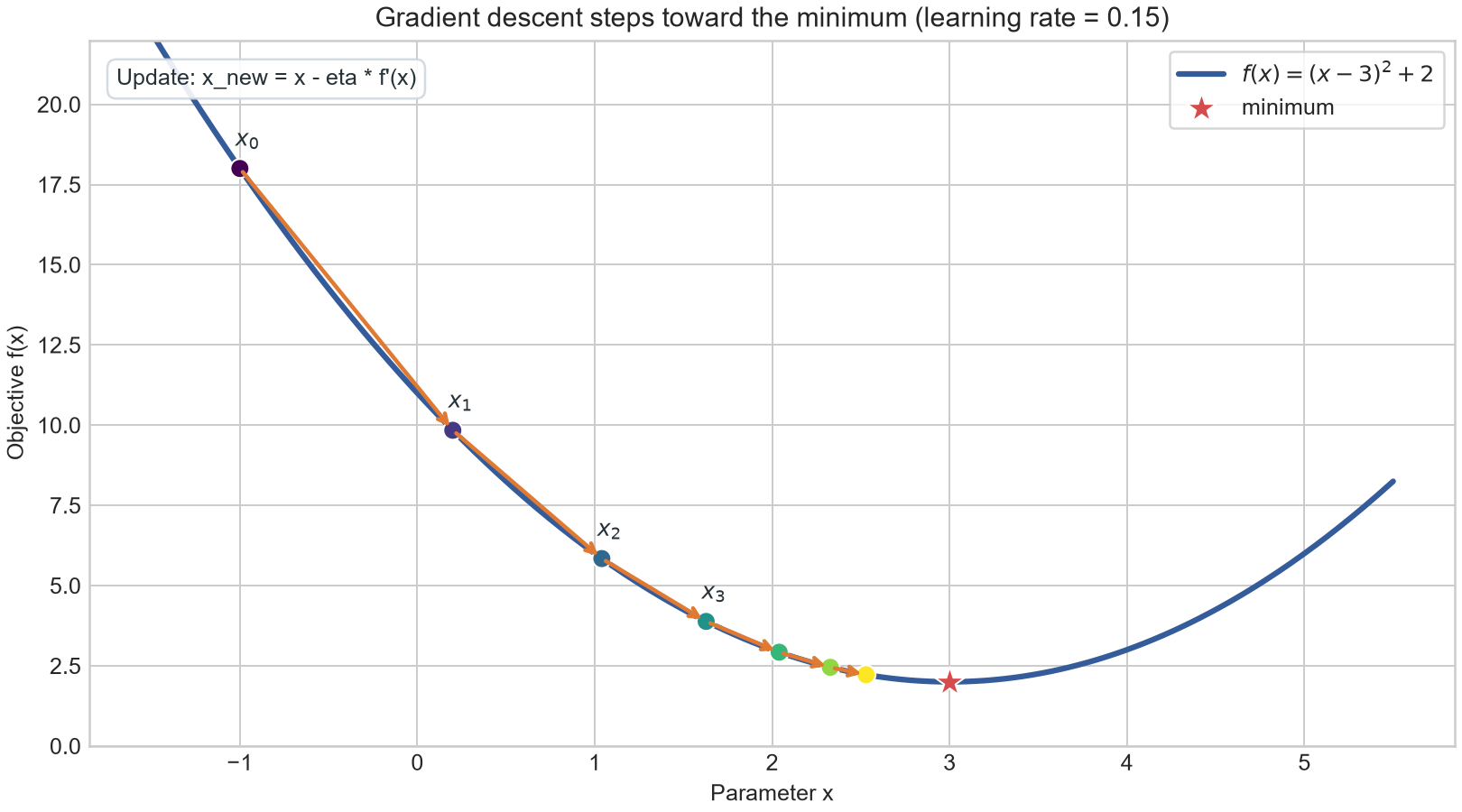
Each step moves opposite the local slope, approaching the minimum of the curve.

The update rule

Suppose we want to minimize a differentiable function \(J(\theta)\), where \(\theta\) may be one parameter or a vector of parameters. Its gradient, \(\nabla J(\theta)\), points in the direction of steepest local increase. Gradient descent moves against it:

where \(t\) is the iteration and \(\eta > 0\) is the learning rate. A small learning rate takes cautious steps; a large one can overshoot the minimum. The appropriate value depends on the scale and curvature of the objective.

For a one-dimensional example, consider

Its derivative is \(f’(x)=2(x-3)\), so the update becomes

The minimum is at \(x=3\). In the notebook, we start at \(x_0=-1\), calculate several updates, and plot the iterates on the curve. The visualization shows each step moving down the bowl toward its minimum.

Linear regression as an optimization problem

Next, we fit a line to data points \((x_i,y_i)\). Our model predicts

where \(w\) is the slope and \(b\) the intercept. We choose the parameters by minimizing mean squared error:

Let \(e_i=wx_i+b-y_i\). Applying the chain rule gives the two gradients:

The Python implementation evaluates those formulas for all examples at once:

def mse_and_gradient(w, b, x, y):
    error = w * x + b - y
    loss = np.mean(error ** 2)
    grad_w = 2 * np.mean(error * x)
    grad_b = 2 * np.mean(error)
    return loss, grad_w, grad_b

Each training step computes the gradients using the current parameters, then updates both:

loss, grad_w, grad_b = mse_and_gradient(w, b, x, y)
w -= learning_rate * grad_w
b -= learning_rate * grad_b

The notebook creates a small deterministic dataset around \(y=2.5x+1\), adds seeded noise, and standardizes the input feature before training. It then plots the observations and fitted line, along with the loss over iterations.

Why feature scaling helps

Gradient descent uses one learning rate for all parameters. If features have very different scales, the loss surface can be stretched: one direction may be steep while another is shallow. A step large enough to make progress in the shallow direction can overshoot in the steep one.

Centering and scaling a feature helps balance those directions. It does not change the underlying predictions; after fitting, the notebook converts the slope and intercept back to the original input scale.

Learning rate: too small, useful, or too large

The notebook compares three learning rates on the same regression problem:

• A small value reduces loss steadily but slowly.
• A useful value makes faster progress while keeping the loss under control.
• A too-large value overshoots and diverges for this example.

The comparison is plotted on a logarithmic loss axis so both slow progress and rapid growth are visible. A learning rate that works on one dataset may not work on another; scaling the inputs and monitoring the loss are practical first steps.

The loss landscape

The regression objective depends on two parameters, \(w\) and \(b\). For every pair of values, we can calculate a loss. A contour plot connects points with equal loss, and an optimization path shows how the parameter pair moves over the landscape:

for _ in range(steps):
    loss, grad_w, grad_b = mse_and_gradient(w, b, x, y)
    w -= learning_rate * grad_w
    b -= learning_rate * grad_b

The notebook overlays this path on the loss contours. For squared-error linear regression, the objective is convex, so every local minimum is global. That guarantee does not apply to arbitrary non-convex objectives such as neural-network losses.

Run the notebook

The Jupyter notebook contains all code needed to reproduce the plots:

1. A one-dimensional loss curve with annotated gradient steps.
2. A synthetic-data scatter plot with the fitted regression line.
3. A training-loss curve and a learning-rate comparison.
4. A contour plot of the two-parameter loss surface with the optimization path.

It uses NumPy and Matplotlib and does not download data. If those packages are not installed in your environment, install them in the Python environment selected by Jupyter:

python -m pip install numpy matplotlib

Takeaways

Gradient descent repeatedly evaluates a gradient and updates parameters in the direction that reduces the objective. The math is compact, but behavior depends on the learning rate, feature scales, and shape of the loss surface. Visualizing the trajectory makes those choices easier to understand—and the notebook lets you change them and observe what happens.